Pipeline Parallelism: The Bubble Problem and Why 8 GPUs Sometimes Trains Slower Than 4
The 8-GPU regression
A distributed systems team at an ML infrastructure company added four GPUs to their training cluster. The original four-GPU setup ran at 92% GPU compute utilisation during forward passes. After the expansion to eight GPUs, utilisation dropped to 61%. Training throughput — tokens processed per second — fell by 18% compared to the four-GPU baseline.
Adding four GPUs made their training slower.
The team had increased their pipeline parallelism degree from PP=2 to PP=4, splitting the model across four pipeline stages instead of two. Each stage held roughly one quarter of the transformer layers. On paper, doubling the pipeline depth should have allowed larger effective batch sizes and higher throughput. Instead, the GPU utilisation charts showed a repeating pattern: high utilisation for a burst, then a dead zone, then another burst, then another dead zone. The dead zones were exactly as long as the bursts.
The dead zone is called the pipeline bubble. It is not a bug. It is an unavoidable consequence of pipeline parallelism mathematics.
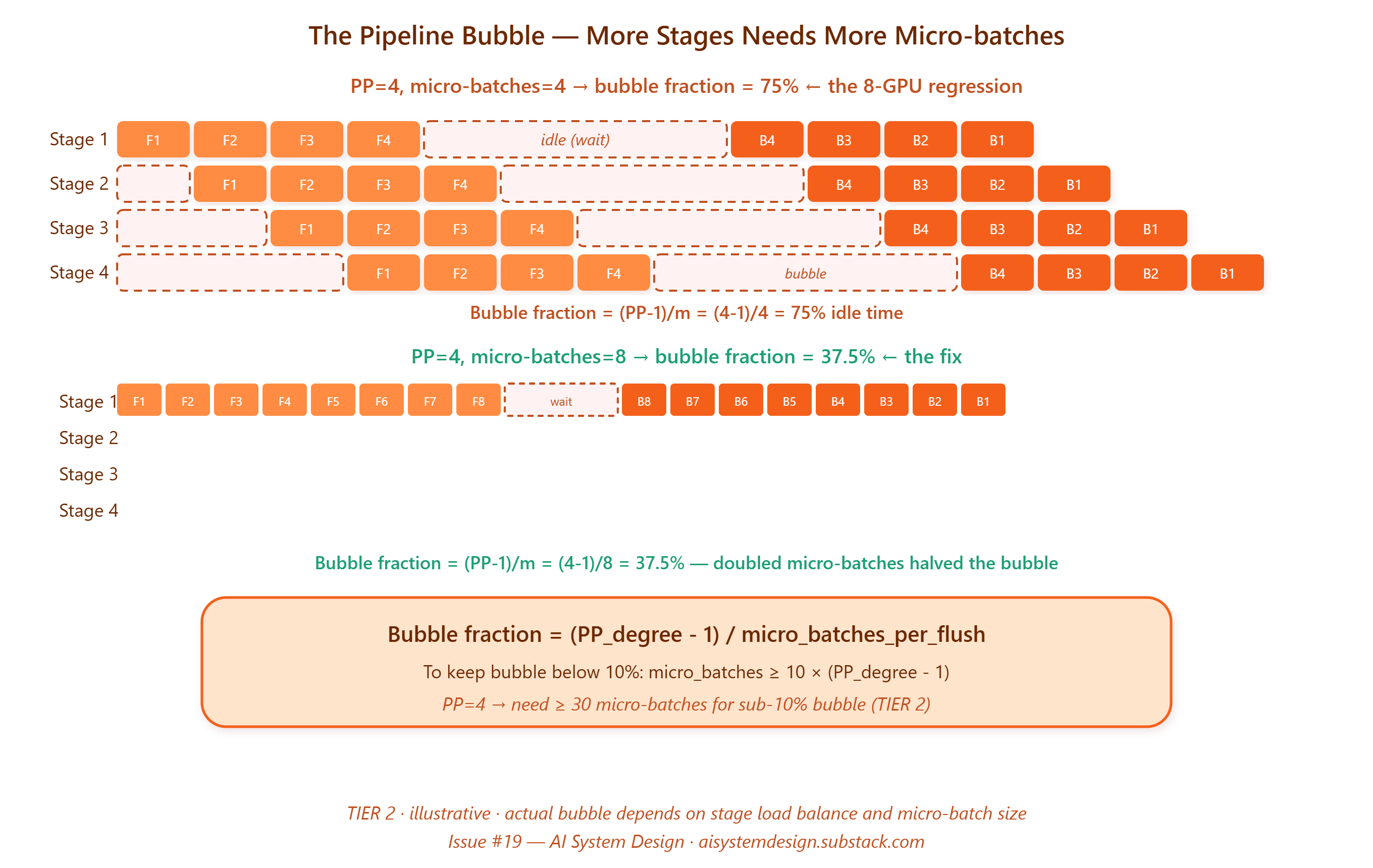
In pipeline parallelism, the model is split into stages. Each stage processes one micro-batch before passing activations to the next stage. Stage 2 cannot start until Stage 1 finishes. Stage 3 cannot start until Stage 2 finishes. This creates a startup latency at the beginning of each batch: Stage 1 must complete its first micro-batch before Stage 2 has anything to do. During this startup, Stages 2, 3, and 4 are idle.
At the end of each batch, the reverse happens in the backward pass. Stage 4 finishes first. It must wait while Stage 3, then Stage 2, then Stage 1 complete their backward passes before the next forward pass can begin. Stages 1, 2, and 3 are idle while Stage 4 waits.
The bubble fraction — the fraction of time that GPUs are idle due to pipeline startup and teardown — is approximately (PP_degree - 1) / micro_batches_per_pipeline_flush (TIER 2). At PP=2 with 8 micro-batches, bubble fraction ≈ 1/8 = 12.5%. At PP=4 with 4 micro-batches, bubble fraction ≈ 3/4 = 75%. The team had increased PP degree without proportionally increasing the number of micro-batches per flush. The bubble ate their throughput.
What the team was missing: the relationship between pipeline depth and the minimum number of micro-batches required to keep all pipeline stages busy.
Why pipeline parallelism breaks the “more stages = more throughput” assumption
The intuition is seductive: if Stage 1 processes a micro-batch while Stage 2 processes the previous one, you get two stages of processing happening simultaneously, effectively doubling throughput. Like a factory assembly line, each station stays busy while work flows through in sequence.
The assembly line analogy is instructive precisely because it reveals where the intuition breaks. Consider a car factory with four assembly stations. Each car takes one hour per station. To keep all four stations busy simultaneously, you need at minimum four cars in progress at once — one at each station. If you only have three cars, Station 4 is always waiting. If you only have two cars, Stations 3 and 4 spend most of their time idle. The pipeline efficiency is limited by how many units you can keep flowing through the system simultaneously.
LLM pipeline parallelism has the same constraint. Each pipeline stage needs a stream of micro-batches flowing through it to stay busy. The minimum number of micro-batches required to fully saturate a PP-stage pipeline is equal to PP_degree. Below this minimum, some stages are always idle waiting for micro-batches to arrive.
Here’s the key thing: pipeline bubble fraction is determined by the ratio of (PP_degree - 1) to micro_batches_per_flush — and the only way to reduce it without reducing PP_degree is to increase the number of micro-batches, which increases memory pressure and may require gradient accumulation.
The pipeline bubble visualised (free)