
How Continuous Batching Cut an AI Startup’s GPU Bill from $40,000 to $6,000 (Without Changing Hardware)
The team that was spending $40,000 a month to serve 200 users
A consumer AI startup had 200 daily active users on their writing assistant. Their monthly GPU bill was $40,000. Their CTO pulled up the GPU utilisation dashboard during a weekly review. The cards were averaging 8% compute utilisation across the day.
They were running four A100 80GB SXM4s. Each was loaded with the model. Each was generating tokens for requests one at a time — receiving a request, running it start to finish, then picking up the next one. While one request was being served, the other three GPUs in the cluster were mostly idle. While that one GPU was serving its request, it was generating about 14 tokens per second. The rest of the time, it was waiting for the next request to arrive.
The GPU cost was real. The GPU work was not. They switched to continuous batching in a single afternoon. Their monthly bill dropped to $6,000. Same model. Same hardware. Same users. The GPU was now generating tokens for 8–12 requests simultaneously instead of 1.
That’s not an optimisation. That’s discovering that the car was running the whole time and nobody was driving it.
Why serving requests one at a time is the same as running a restaurant kitchen for one table
Most people understand intuitively how a restaurant kitchen works at scale. There are eight burners. A good chef runs all eight simultaneously — different dishes at different stages. If a chef cooked one order completely before starting the next, the kitchen would produce roughly the same number of meals per hour as a single burner, and seven of them would be cold and unused.
Early LLM serving systems worked exactly like that single-burner chef. A request arrived, the GPU processed it from the first token to the last, the response was returned, and only then did the next request get loaded. This is called static batching at the request level. It seems safe and simple. It wastes almost everything.
The reason it wastes so much is the shape of LLM inference. Generating a response has two phases. The first phase — prefill — processes the entire input prompt in one pass. It’s fast, compute-intensive, and takes roughly the same time regardless of how many requests you batch together. The second phase — decode — generates output tokens one at a time, one per step, and is slow because it’s memory-bound as we covered in Issue #01.
If you process requests one at a time, the decode phase of Request A consumes one GPU step per output token. While that step runs, Request B is queued. Request B’s user is waiting. The GPU is doing one thing at a time when it could be doing dozens.
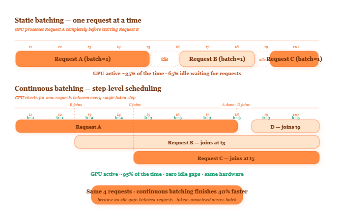
Continuous batching solves this by making a simple observation: between every single token generation step, the GPU is free to check whether any new requests are ready to start. If they are, add them to the batch for the next step. If any existing requests just finished, remove them from the batch.
Here’s the key thing: continuous batching operates at the step level — between every single token — not at the request level. This means the batch composition changes constantly, and the GPU is always working on as many requests as will fit in memory simultaneously.
Github Link:
https://github.com/sysdr/AISysDesign-Labs/tree/main/inference-vault/issue-07
How the batch changes between every single token step
What the scheduler actually does between every token step
The mechanism works at the iteration level — meaning between every single token generation step, not between requests.
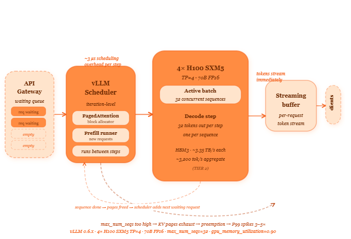
Here’s the exact sequence. The GPU finishes one decode step. It has just produced one new token for each active sequence in the batch. Before it starts the next step, the vLLM scheduler runs four operations in sequence. First: it checks which sequences just generated their end-of-sequence token and removes them from the batch, returning their KV cache pages to the free pool. Second: it checks the waiting queue for new requests. Third: for each waiting request that can be accommodated — meaning there are enough free KV cache pages — it runs a prefill pass to process the input prompt and adds the sequence to the active batch. Fourth: it launches the next decode step with the updated batch.
This entire scheduling cycle happens between every single token generation step. On an H100 SXM5 generating 3,000 tokens per second aggregate across a batch of 32, that’s 3,000 scheduling decisions per second. Each one takes microseconds. The overhead is negligible compared to the token generation time.
The result: no request ever waits for another request to finish. A new request arriving while 20 others are mid-generation joins the batch on the very next step — as long as KV cache pages are available.
python
# vLLM 0.6.x — configure continuous batching parameters
# Verify argument names at vllm.readthedocs.io/en/latest/serving/engine_args
from vllm import LLM, SamplingParams

llm = LLM(
    model="meta-llama/Meta-Llama-3.1-70B-Instruct",
    tensor_parallel_size=4,
    max_num_seqs=64,           # ← maximum concurrent sequences in the batch
    max_num_batched_tokens=8192, # ← max tokens processed per step (prefill + decode)
    gpu_memory_utilization=0.90,
)

# The scheduler runs automatically — you don't call it explicitly.
# Generate requests concurrently and vLLM handles batching internally.
sampling_params = SamplingParams(temperature=0.7, max_tokens=256)
prompts = ["Explain CXL memory pooling.", "What is PagedAttention?"]
outputs = llm.generate(prompts, sampling_params)
# Both prompts are batched together internally
The most common wrong assumption: engineers think continuous batching means waiting to collect a full batch before processing. It doesn’t. It means processing whatever is ready right now and adding more as they arrive. A batch of 1 starts immediately. A batch of 32 happens to have 32 sequences ready at the same time. The scheduler never waits.
The second wrong assumption: engineers think the GPU processes all sequences in the batch at the same speed, so a very long request blocks shorter ones. This is partially true for memory — a long request holds KV cache pages until it finishes — but it’s not true for scheduling. Short requests that arrive mid-stream join the batch immediately and finish whenever their output is done, regardless of where longer co-batched requests are in their generation. The long request doesn’t block the short one. They run in parallel on the same GPU, each producing one token per step.
Where the scheduler lives in a production inference cluster
What makes continuous batching work — and what breaks it
Two upstream decisions determine whether continuous batching delivers its promised gains.
First: your serving framework must implement iteration-level scheduling. This is not the same as request-level batching, which most naive serving implementations use. Request-level batching collects a group of requests, processes them all together from start to finish, then starts the next group. Iteration-level scheduling adjusts the batch between every single token step. vLLM 0.6.x implements iteration-level scheduling by default. TGI implements it. Older frameworks like simple FastAPI wrappers around model.generate() do not — they process one request at a time. If you’re running a custom serving stack built around HuggingFace’s generate() call without modification, you almost certainly have request-level batching and are leaving most of your throughput on the floor.
Second: your max_num_seqs setting must be tuned to your KV cache capacity. This parameter tells vLLM the maximum number of sequences it should run concurrently. Setting it too low means the batch never reaches the size that amortises weight loading effectively — throughput suffers. Setting it too high means the KV cache page pool runs out, the scheduler starts preempting sequences, and P99 latency spikes by 3–5×. The right value depends on your average sequence length, your model size, and your HBM capacity. Start at 32, measure KV cache utilisation via vllm:gpu_cache_usage_perc, and tune from there.
When both are right, two downstream effects compound. Aggregate throughput rises 8–15× compared to single-request serving on the same hardware — because the weight loading cost is amortised across the full batch on every step rather than paid once per request (TIER 2 — varies with batch size, sequence length distribution, and model size). And cost per token drops by the same factor, because you’re generating far more tokens per GPU-hour than you were before.
When max_num_seqs is misconfigured high, the downstream failure is specific: vLLM’s preemption count metric vllm:num_preemptions_total starts rising, individual requests that get preempted experience latency spikes of 200–500 ms or more as their KV cache is swapped to CPU RAM and back, and P99 diverges from P50 dramatically. The median experience looks fine. The tail experience is terrible. Both Prometheus and vLLM’s built-in metrics endpoint expose num_preemptions_total directly — watch it.
Which configuration to reach for first
The decision is simpler than most engineers expect. Continuous batching with sensible defaults handles the vast majority of production workloads. The real decisions are around how aggressively to tune max_num_seqs and whether your traffic pattern is uniform enough to set it statically.
START: Are you currently serving requests one at a time?
│      (check: is your framework calling model.generate() per request?)
├── YES → Switch to vLLM 0.6.x immediately.
│         Why: iteration-level scheduling is the single highest-leverage
│         change available. 8–15× throughput gain at zero model or
│         hardware cost is typical. (TIER 2 — varies with load)
│         Start with defaults: max_num_seqs=32, gpu_memory_utilization=0.90.
└── NO (already using vLLM or TGI) →
    Is vllm:gpu_cache_usage_perc above 90% during peak?
    ├── YES → Is vllm:num_preemptions_total growing during peak?
    │   ├── YES → Reduce max_num_seqs by 20%, wait 24h, re-measure.
    │   │         Why: you're exhausting the KV cache pool — preemptions
    │   │         are spiking your P99 even if P50 looks fine.
    │   └── NO  → Increase gpu_memory_utilization by 0.02 (up to 0.95).
    │             Why: you have headroom but your pool is near-full —
    │             a small increase gives you more pages without risk.
    └── NO (cache usage below 90%) →
        Is throughput below your target despite low cache usage?
        ├── YES → Increase max_num_seqs to 64, then 128.
        │         Why: you have KV cache space but aren't filling the batch.
        │         More concurrent sequences = better amortisation.
        └── NO  → Your continuous batching is well-tuned. No changes needed.
                  EDGE CASE: If request arrival is bursty, consider chunked
                  prefill (--enable-chunked-prefill in vLLM 0.6.x) to prevent
                  large prefill passes from blocking decode for too long.
The batch size economics that made the startup’s $40,000 bill fall to $6,000
Here’s the arithmetic the startup was living inside.
At batch size 1, the GPU loads roughly 140 GB of weights per token (for a 70B FP16 model at TP=1 on one A100 80GB SXM4) and produces 1 token. Weight load cost per token: 140 GB.
At batch size 32, the GPU loads roughly 140 GB of weights per step and produces 32 tokens simultaneously — one per sequence. Weight load cost per token: 140 GB ÷ 32 = 4.375 GB.
That’s a 32× reduction in weight loading cost per token. Not a 32× improvement in raw speed — because the memory wall still bounds the absolute rate — but a 32× improvement in the ratio of useful work to memory bandwidth consumed. The GPU generates 32× more tokens for the same bandwidth expenditure.
For the startup, this meant the same four A100s that were generating tokens for roughly 14 hours per day of equivalent useful work at batch size 1 were now generating tokens continuously. Monthly cost dropped from $40,000 to $6,000 not because the GPUs got cheaper but because they stopped being idle.
This is also why the cost-per-token metric is the right thing to watch — not GPU utilisation percentage alone. GPU utilisation at 95% during a continuous batching run means you’re generating tokens constantly. GPU utilisation at 95% during a single-threaded inference loop might just mean one request is being processed very intensively while a queue of others waits. You need both the utilisation number and the tokens-per-GPU-hour number together.
bash
# Compute tokens per GPU-hour from vLLM metrics
# Requires Prometheus scraping vLLM's /metrics endpoint
# Verify metric names at vllm.readthedocs.io/en/latest/serving/metrics

# Query: tokens generated per second
curl -s http://localhost:8000/metrics | grep "vllm:generation_tokens_total"

# Divide by number of GPUs to get tokens per GPU per second
# Multiply by 3600 to get tokens per GPU-hour
# Compare against your target: at batch=32 on 70B, expect 800-1200 tok/GPU/hr (TIER 2)
# At batch=1 on 70B, expect 50-80 tok/GPU/hr (TIER 2)
Why the iteration-level scheduling insight is permanent
The economic argument for continuous batching is rooted in the same physics as the memory wall. Every time the GPU loads the model weights for a decode step, it can produce one token per active sequence in the batch. Weight loading costs are fixed per step regardless of batch size — because the weights are the same size whether you run 1 sequence or 64. So producing more output per fixed-cost step is always economically rational.
This argument doesn’t change with hardware generation. H100 SXM5 has more bandwidth than A100. Both benefit from continuous batching by the same ratio — the batch size determines how many tokens you produce per bandwidth expenditure, not the absolute bandwidth. B200 with HBM3e benefits by the same ratio again.
The specific implementation evolves. DistServe and the disaggregated prefill/decode architecture — shipping in various forms across vLLM and SGLang — takes continuous batching further by running prefill and decode on separate GPU pools. Prefill is compute-bound and benefits from large batches of prompts processed together. Decode is memory-bound and benefits from the continuous batching approach described here. Separating the two means neither blocks the other — a long prefill no longer delays a mid-generation decode step, and vice versa. This is the next evolution, and it’s built directly on the continuous batching foundation.
What changes in the next 12–18 months: hardware-disaggregated serving becomes standard. The prefill GPUs and the decode GPUs are different pools with different optimisation targets. Teams that understand why prefill and decode have different bottlenecks — and continuous batching is the gateway to understanding that distinction — will implement disaggregated serving when it matters and not before.
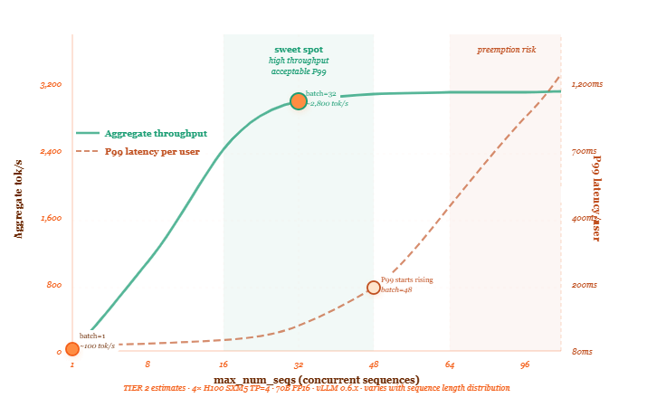
The throughput vs latency tradeoff at different batch sizes
The assumption that a bigger batch always means worse latency per user
The assumption is that serving more users simultaneously means each user waits longer for their response. This feels true. It is mostly wrong — and understanding exactly where it’s wrong and where it becomes right is the practical skill.
At batch size 1, a user’s first token arrives after one decode step — roughly 30–50 ms on a 70B model at TP=4 on H100 SXM5 (TIER 2). At batch size 32, a user’s first token still arrives after one decode step — the same 30–50 ms. The decode step takes slightly longer because 32 tokens are being produced instead of 1, but the increase is small because the step is memory-bound and dominated by weight loading time, not compute time. Time to first token barely changes from batch 1 to batch 32.
What does increase is time to last token — the total time for the full response to arrive. Because the GPU is handling 32 sequences simultaneously, each sequence gets one token per step. If Request A needs 200 tokens and Request B needs 50 tokens, Request B finishes after 50 steps and Request A after 200 steps, regardless of batch size. The total wall-clock time per request is proportional to the output length, not the batch size. At larger batch sizes, each step takes slightly longer — but not proportionally longer.
What breaks at high batch size is KV cache exhaustion. When you push max_num_seqs so high that the free page pool runs out, the scheduler begins preempting sequences — swapping their KV cache to CPU RAM and restarting them later. Those preempted sequences experience latency spikes of 200–500 ms or more while their pages are swapped back in. This is the source of the P99 spike. It has nothing to do with batch size per se — it’s about KV cache management.
The correct way to think about it: increasing batch size hurts P99 latency only when it forces KV cache exhaustion and preemption. Up to that point, it has a small and manageable effect on total response time per request, while dramatically improving throughput and cost per token. The dial to watch is vllm:num_preemptions_total, not batch size itself.
[ FOR DECISION MAKERS ]
What this affects: Your cost per API call, how many users your current GPU cluster can serve, and whether you need to buy more hardware to meet your traffic targets.
What it costs to get wrong: The startup in this issue’s opening was spending $40,000 per month to serve 200 users because their serving framework processed one request at a time. The cost was not driven by traffic volume or model size — it was driven by a configuration choice. The same 200 users on the same hardware with continuous batching cost $6,000 per month. The difference between $40,000 and $6,000 is a framework switch and an afternoon of tuning.
One question to ask your engineering team: “How many requests are we serving simultaneously on each GPU right now, and what framework handles the request batching? If the answer is one at a time or an old custom wrapper, we should look at switching to vLLM or TGI before we consider buying more hardware.”
Measure your current batch size before changing anything
TOOL:           vLLM 0.6.x Prometheus metrics endpoint
                (verify metric names at vllm.readthedocs.io/en/latest/serving/metrics)
RUN:            # Expose the metrics endpoint (enabled by default in vLLM)
                # Then query during a live traffic window:
                watch -n 5 'curl -s http://localhost:8000/metrics | \
                  grep -E "num_requests_running|gpu_cache_usage|num_preemptions"'

                # Key numbers to capture during peak traffic:
                # vllm:num_requests_running — current active batch size
                # vllm:gpu_cache_usage_perc — KV cache pool utilisation
                # vllm:num_preemptions_total — preemption count (bad if rising)
CHANGE:         Adjust max_num_seqs in your vLLM startup command:
                --max-num-seqs 32 → 64 → 128 in 24h increments
LOOK FOR:       num_requests_running below 8 during peak = under-batching
                gpu_cache_usage_perc above 90% = near KV exhaustion
                num_preemptions_total rising = reduce max_num_seqs now
EXPECTED RANGE: Well-tuned continuous batching keeps gpu_cache_usage_perc
                between 60–85% during peak with zero preemptions. (TIER 2)
If num_requests_running is consistently below 8 during peak traffic even at high max_num_seqs, your problem is not batch size — you don’t have enough concurrent users. In that case speculative decoding (Issue #06) is more relevant than continuous batching tuning.
If continuous batching comes up in a system design interview
THE QUESTION:
Your company serves a 70B model to internal enterprise users — roughly 500
people sending requests during business hours, maybe 40 concurrent at peak.
Current setup: a single A100 80GB SXM4, single-request serving via a FastAPI
wrapper around model.generate(). Users are complaining it's slow. You have
budget to either upgrade to H100 SXM5 hardware or spend engineering time.
What do you recommend?

WHAT A STRONG ANSWER COVERS:
- Immediately identifies the serving architecture as the problem — single-
  request serving at 40 concurrent users means 39 users are always queued
  while 1 is being served, even if that GPU is fast
- Recommends switching to vLLM with continuous batching before any hardware
  change — the throughput gain is 8–15× on identical hardware (TIER 2)
- Notes that a 70B model does not fit on a single A100 80GB SXM4 in FP16
  (140 GB weights > 80 GB HBM) — the current setup must be using
  quantisation or the question has a different model assumption

WHAT MAKES IT A GREAT ANSWER:
A senior engineer checks the hardware feasibility first — 70B FP16 on one
A100 80GB is impossible, so they clarify whether the model is quantised,
uses tensor parallelism, or is actually a smaller model — before recommending
anything. Answering the design question without catching the hardware
impossibility is the gap between a senior and a staff-level answer.

FOLLOW-UP QUESTIONS:

Q2: "Let's say the model is a 13B FP16 model, fits on one A100 80GB.
     You switch to vLLM. Three weeks later, during a product launch,
     peak concurrent users hits 200. P99 latency spikes to 4 seconds.
     What happened and what do you do?"
→ Good answer adds: at 200 concurrent users on max_num_seqs=32, the
  waiting queue is growing faster than requests complete — the GPU is
  at throughput capacity, not just batching inefficiency; first add a
  second A100 instance (horizontal scaling) before increasing max_num_seqs
  beyond KV cache capacity; separate the concurrency problem from the
  batching problem

Q3: "You have 4 A100 80GB SXM4s available. Should you run 4 separate
     vLLM instances serving the 13B model, or 1 vLLM instance across
     all 4 GPUs using tensor parallelism?"
→ Good answer adds: 4 independent instances give 4× the aggregate
  throughput and better fault isolation — if one fails, 3 still serve;
  tensor parallelism across 4 GPUs reduces per-request latency but gives
  the same aggregate throughput while adding NVLink coordination overhead;
  for a 13B model that fits on one GPU, 4 independent instances is almost
  always the right answer — tensor parallelism is for models that don't fit

Q4: "One of your 4 instances is producing outputs that differ from the
     other 3 for identical prompts. How do you diagnose it?"
→ Good answer adds: check whether that instance has a different
  gpu_memory_utilization setting causing more aggressive KV preemption —
  preempted and restarted sequences can produce different outputs if
  temperature > 0 and the random seed changes on restart; check vLLM
  version on that instance; check whether that GPU has ECC errors via
  nvidia-smi --query-gpu=ecc.errors.corrected.volatile.total
Where the foundational work is
→ Orca: A Distributed Serving System for Transformer-Based Generative Models
  — Yu et al., OSDI 2022
  The paper that introduced iteration-level scheduling for LLM serving.
  Section 3 describes the selective batching and iteration-level scheduling
  mechanism that vLLM and TGI implement. This is where the idea originated.

→ Efficient Memory Management for Large Language Model Serving with
  PagedAttention — Kwon et al., SOSP 2023
  Section 4 describes how PagedAttention enables continuous batching
  by making KV cache allocation incremental — the two mechanisms are
  designed to work together and this paper explains why.

→ vLLM documentation: engine arguments
  vllm.readthedocs.io/en/latest/serving/engine_args.html
  The authoritative reference for max_num_seqs, max_num_batched_tokens,
  gpu_memory_utilization, and enable_chunked_prefill. More useful than
  any blog post on the topic.

→ Sarathi-Serve: Efficient LLM Inference by Piggybacking Decodes with
  Chunked Prefills — Agrawal et al., OSDI 2024
  The paper behind vLLM's chunked prefill feature. Explains why chunked
  prefill reduces P99 latency spikes from long prompts. Read this if
  your workload has high prompt length variance.

→ DistServe: Disaggregating Prefill and Decoding for Goodput-Optimized
  Large Language Model Serving — Zhong et al., OSDI 2024
  Describes the next evolution of continuous batching — separate GPU
  pools for prefill and decode. The logical continuation from where
  this issue ends.
The car was running the whole time
The startup’s GPUs were on. The fans were spinning. The electricity meter was running. The model was loaded. And 92% of the time, nothing was being generated.
This is not a rare failure mode. It’s the default configuration for any team that took a model off HuggingFace, wrapped it in a web server, and called it production. The model works. The serving architecture doesn’t.
Engineers who understand continuous batching check the batch size before they check the hardware. Not “is this GPU fast enough?” but “is this GPU ever working on more than one thing at a time?” If the answer is no, the hardware question is premature. The economics of LLM serving are almost entirely determined by how many tokens you produce per unit of fixed-cost weight loading. Everything else is secondary to that ratio.
The bill went from $40,000 to $6,000 in one afternoon. The car had been running the whole time. Nobody was driving it.